In this tool, you can compute the surface and volume of the Tag images for the selected frames. These results can be displayed numerically and in a graph and can be written to 2 different files: a spreadsheet compatible file or an ASCII text file.
By default the tool display the surfaces (in cm2) and volumes (in cm3) for all the tag values existing in the selected frames. You can change the units for these measurements with the "Units" tool, and you can change the list of displayed values with the "Results: Display" command.
WARNING:
|
|
|
From the Graphic Interface
|
|
|
|
Some of the values computed by this tool are displayed in this window. If you want access to all the values computed, you need to open a secondary window with the "Window Values" button. You can control which of the values are displayed with the command line. By default, the surfaces and volumes are displayed.
|
|
|
The values computed are: •"Surface Units", The surface of each TAG in surface units (see the Units tool) •"Volume Units", The volume of each TAG in volume units (see the Units tool) •"Surface Pixel", The surface of each TAG in pixels •"Volume Voxel", The volume of each TAG in voxels •"GLI Mean", The mean value of the pixel under each TAG in the pixel's units •"GLI Min", The minimum value of the pixel under each TAG in the pixel's units •"GLI Max", The maximum value of the pixel under each TAG in the pixel's units •"GLI SD", The standard deviation of the values of the pixel under each TAG.
The values that are not selected to be saved in the result files will be displayed in grey. This can be changed either from the configuration menu or through the command line.
Only one such window can exist at any time, clicking this button while the window is already created will pop the associated window on top of the other windows.
|
|
|
Window Graph |
Only one such window can exist at any time, clicking this button while the window is already created will pop the associated window on top of the other windows.
|
|
If you know what is the relationship between pixel values and something else, you can add a calibration file that will define this relationship. For example, if you know how to compute a tissue density from the CT Housfield units (HU), you can use a calibration file to let the program know about this. In this way, the mean, min and max values will be in densities instead of HU.
|
|
|
Clicking this button will open a configuration menu. In this menu you will be able to specify the content and form of the result files you can create from this tool. The configuration menu is described in more detail further down.
|
|
|
Create a result file. The results can be either in standard ASCII text, or in a tabulated form compatible with Excel. You can set the default for this with the configuration menu, or changing the "save as type" parameter in the confirmation pop-up window.
|


|
|
|
|
Result files can either be in plain ASCII text (compatible with notepad or any text editors) or in "DB file", a tabulated form, compatible with Excel or most spreadsheet programs.
|
|
|
You can have 3 optional headers in the files you created:
The Patient Info header
For each patient used in creating the file we will have (if the information is present in the image's header): •Patient Name •Patient ID •Patient sex •Date of Birth •Patient weight (Kg) •Patient height (m)
|
|
|
|
The Scanner Info header
For each scanner used in creating the file we will have (if the information is present in the image's header): •Modality •Manufacturer •Model
|
|
|
The Image Info header
For each image used in creating the file we will have (if the information is present in the image's header): •Resolution X Y •Pixel Dim. X Y Z (mm) •Horiz. Dir. X Y Z •Vert. Dir. X Y Z
|
|
Saved Measures |
You can select which of the available measures you want to save in your result files.
|
|
Float Fraction |
You can specify whether you want the fractions in your floating point values to be delimited by a dot (".") (example:12.34) or a comma (",") (example: 12,34). By default it is the dot.
|
|
Cell Delimiter |
You can specify the character you want to use to mark the end of a cell in your spreadsheet result files. By default it is the "tab" character.
|
|
Cell Filler |
You can specify what should be placed in cells that have no values. For example, in a result file for multiple frames, if a TAG is not present in all the frames, then in some cells we will not have surfaces and volumes for it.
|
|
Default Path |
You can specify the default path for the results files. There is only one "default path" parameter in sliceOmatic, so by default, this value is set to the path of the last file read or written.
|
|
Default Name |
You can set a default name for your result files.
|
|
Cancel |
Close the configuration menu without saving any of the changes you just made.
|
|
Accept Changes |
Accept the changes you made and close the configuration menu. Please note that these changes only affect the current invocation of sliceOmatic. If you want to save the changes for future invocations of the program, you need to use the "Script Save As..." option of the File menu. |

The surface area covered by a Tag value is computed by multiplying the number of pixels of that value by the surface area of one pixel.
Computing the volume of a Tag value for one image is fairly simple. We compute the surface area covered by the Tag value and multiply by the image thickness. For multiple images, a problem arises if the images overlap or if there are gaps between them.
Note:
|
|
|
Using the notation:
= position in Z of the image A
|
|
ZA |
= position in Z of the image A |
|
|
NA |
= number of pixels of a certain Tag value in image A |
|
|
PA |
= surface of a pixel in image A |
|
|
SA |
= surface covered by a Tag value on the image A (= NA PA) |
|
|
TA |
= thickness of image A |
|
|
AB |
= gap or overlap between the two images A and B |
|
|
VAB |
= volume of a Tag value between the two images A and B |
The gap ∆ between two images A and B is computed as follows:
∆AB = ABS(ZA - ZB) - (½TA + ½TB)
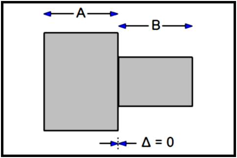
Depending on the value of ∆, there are 3 possibilities when computing the volume between 2 images:
|
|
∆ = 0 |
There is no gap, and the computation of the volume of the Tag value between A and B is straightforward:
VAB = ½TASA + ½TBSB
|
|
|
|
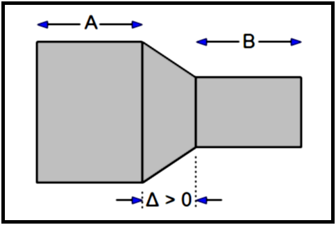
∆ > 0 |
There is a gap between the slices and we have to interpolate the volume in the gap. This volume will be approximated by a truncated pyramid joining the volumes of both slices.
VAB = ½TASA + ½TBSB + ∆AB (1/3 ABS(SA - SB) + MIN(SA, SB))
|
|
|
|
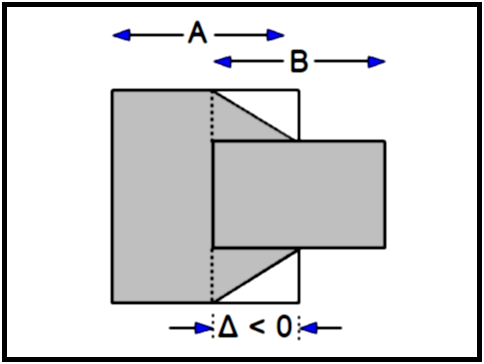
∆ < 0 |
The images overlap and we have to compute the volume in this overlap region. The volume in the region without overlap is computed as before, and in the overlap we will again use the truncated pyramid.
VAB = (½TA + ½∆AB) SA + (½TB + ½∆AB) SB - ∆AB (1/3 ABS(SA - SB) + MIN(SA, SB))
|
|
Example: We will compute the volume of the Tag value 1 for 4 images:

|
|
All slices are 10.0 mm thick All pixels are 0.25 mm2
|
(Ta to TD = 10.0) (PA to PD = 0.25) |
|
|
Image A: |
|
|
|
has 400 pixels of Tag value 1 is positioned at Z = 100.0 |
(NA = 400) (ZA = 100.0) |
|
|
image B: |
|
|
|
has 300 pixels of Tag value 1 is positioned at Z = 110.0 |
(NB = 300) (ZB = 110.0) |
|
|
image C: |
|
|
|
has 500 pixels of Tag value 1 is positioned at Z = 115.0 |
(NC = 500) (ZC = 115.0) |
|
|
image D: |
|
|
|
has 600 pixels of Tag value 1 is positioned at Z = 130.0 |
(ND = 600) (ZD = 130.0) |
First, we compute the surface area covered by the Tag value 1 for the 4 images:
SA = NA PA = 400 * 0.25 = 100 mm2
SB = NB PB = 300 * 0.25 = 75 mm2
SC = NC PC = 500 * 0.25 = 125 mm2
SD = ND PD = 600 * 0.25 = 150 mm2
Then we compute the volume covered by the Tag value 1. This computation is divided in 5 steps:
• Half the volume of image A: (from Z=95 to Z=100)
|
|
VA |
= ½TA SA |
|
|
|
= ½ 10.0 * 100 |
|
|
|
= 500 mm3 |
• The volume between A and B: (from Z=100 to Z=110)
the value of ∆ is:
|
|
∆AB |
= ABS(ZA - ZB) - (½ TA + ½ TB) |
|
|
|
= ABS(100 - 110) - (½ * 10 + ½ * 10) |
|
|
|
= 0 mm |
there is no gap! The volume is:
|
|
VAB |
= (½TA SA) + (½TB SB) |
|
|
|
= ( ½ 10.0 * 100) + (½ 10.0 * 75) |
|
|
|
= 875 mm3 |
• The volume between B and C: (from Z=110 to Z=115)
the value of ∆ is:
|
|
∆BC |
= ABS(ZB - ZC) - (½ TB + ½ TC) |
|
|
|
= ABS(110 - 115) - (½ 10 + ½ 10) |
|
|
|
= -5 mm |
the images overlap by 5 mm! The volume is:
|
|
VBC |
= (½TB + ½∆BC) SB + (½TC + ½∆BC) SC - ∆BC (1/3 ABS(SB - SC) + MIN(SB, SC)) |
|
|
|
= ((½ * 10.0 + ½ * -5) * 75) + ((½ * 10.0 + ½ * -5) * 125) - -5 * ( 1/3 ABS(75 - 125) + MIN(75, 125) ) |
|
|
|
= 187.5 + 312.5 - -5 * (1/3 * 50 + 75) |
|
|
|
= 958.33 mm3 |
• The volume between C and D: (from Z=115 to Z=130)
the value of ∆ is:
|
|
∆CD |
= ABS(ZC - ZD) - (½ TC + ½ TD) |
|
|
|
= ABS(115 - 130) - (½ 10 + ½ 10) |
|
|
|
= 5 mm |
there is a 5 mm gap! The volume is:
|
|
VCD |
= ½TCSC + ½TDSD + ∆CD (1/3 ABS(SC - SD) + MIN(SC, SD)) |
|
|
|
= ( ½ 10.0 * 125) + (½ 10.0 * 150) + 5 * (1/3 ABS(125 - 150) + MIN(125, 150)) |
|
|
|
= 625 + 750 + 5 * (1/3 25 + 125) |
|
|
|
= 2041.66 mm3 |
• Half the volume of image D: (from Z=130 to Z=135)
|
|
VD |
= ½TD SD |
|
|
|
= ½ 10.0 * 150 |
|
|
|
= 750 mm3 |
The total volume is:
|
|
V |
= VA + VAB + VBC + VCD + VD |
|
|
|
= 500 + 875 + 958.33 + 2041.66 + 750 |
|
|
|
= 5125 mm3 |
The mean value is computed as:
Sum of all pixel values / Number of pixels = Σxi / n
The standard deviation is computed using:

From the Display Area
There is no Display Area interaction specific to this tool.
From the Keyboard
There is no keyboard interface specific to this tool.
From the Command Line
System Variables defined in this tool:
|
|
$RESULT_BACKWARD |
(U8) |
Backward compatibility flag (1=compatible with 4.3) |
|
|
$RESULT_NAME |
(A,S) |
Array of result computation name |
|
|
$RESULT_UNIT |
(A,S) |
Array of result computation units |
|
|
$RESULT_ENABLE |
(A,C8) |
Array of flag for the display/output of the result computations (0x01=in output file, 0x02=displayed) |
Text commands defined in this tool:
Results: Backward (on|off|toggle)
Enable or disable the backward compatibility mode. If enable, the database results will have a "frame number" column, and also a column for each empty tag.
Results: Calib (on|off|toggle)
Enable or disable the calibration of the pixel values.
Results: Calib File file_name
Read a calibration file. The calibration file is a script file containing commands specific to the pixel calibration. The commands used in the calibration file are explained further down.
Results: Display t_measure (on|off|toggle)
Enable or disable the display of the measures matching the template "t_measure" in the tool's window. By default, only the "Surface Units" and "Volume Units" measures are displayed.
Results: Enable t_measure (on|off|toggle)
Enable or disable the saving of the measures matching the template "t_measure" in the result files. By default, only the "GLI Variance" measure is disabled.
Results: Measure List
list the names of all the measures performed by this tool. These names can then be used in the "results: enable" and "results: display" commands
Results: Name string
Specify a default name for the result file.
Results: Type (text|db)
Specify a default file type for the result file. The choice is between "db" (spread sheet format) or "text" (simple ASCII text format).
Results: Write [text|db] file_name
Write the surface/volumes to the result file "file_name", in either "db" (spread sheet format) or "text" (simple ASCII text format). If no format is specified, the default value is used.
The calibration file is a script file containing commands specific to the pixel calibration.
Results: Calib Units string
Specify the name of the new units described by the calibration data
If the relationship between the GLI pixel values and the new calibrated values is a simple linear ,transformation, then we can express the calibration with 2 values: offset and scale:
new value = (GLI_Value + offset) * scale
Results: Calib Offset value
Specify the offset of the calibration curve (new value = (GLI_Value + offset) * scale).
Results: Calib Scale value
Specify the scale of the calibration curve (new value = (GLI_Value + offset) * scale).
If the relationship is more complex, we express the calibration with a series of point on calibration curve. All GLI values not specifically defined will be linearly interpolated or extrapolated from the values specified.
Results: Calib Point val_GLI val_new
Specify a point on the calibration curve.