This mode is used to compute the ratio of metabolites in an MR Spectroscopy acquisition.
This ratio is computed by dividing the area of some metabolite peaks by the area of others. In order to do this, the program has to make a series of computations.
The raw data received by the module are a set of complex points acquired by the scanner. On these raw points, the following operation can be performed:
|
|
•Apodization |
An exponential or linear apodization filter can be applied to the time domain data. |
|
|
•Zero Filling |
The time domain data can be expanded by adding zeros at the end of the data. |
|
|
•Phase correction |
(not implemented at this time). |
We then compute a FFT to change from the time domain to the frequency domain.
Once in the frequency domain, we perform the following steps:
|
|
•Baseline removing |
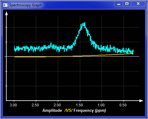
A first baseline approximation is computed to use as a starting point in the peak fitting computation. You have a choice between a power series or a Fourier series. You can also select the number of terms in the series. |
|
|
•Filtering |
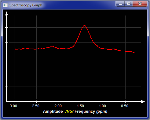
This step is only used because the next step (Water peak detection) is preformed on the filtered data. The filtered data is not use for any other computation but it can be displayed in the Plot Window. |
|
|
•Water peak detection |
This step is used to compute the Hz to ppm scaling. |
|
|
•Peak fitting |
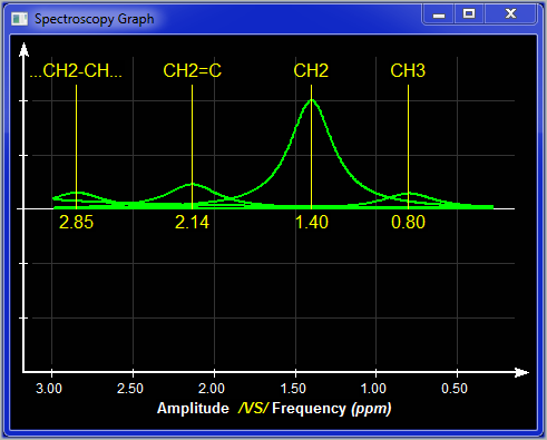
The peak defined in a peak table are fitted to the data curve using a Gauss-Newton least square algorithm. The baseline is also re-compute along with the peaks to get better results. |
|
|
•T1/T2 Correction |
The peak surfaces are corrected for T1/T2 (not implemented at this time). |
|
|
•Peak ratio |
The ratio of the surfaces of some of the fitted peaks is computed. Which peaks' surfaces are in the numerator and which are used in the denominator is set in the peak table.
|
For each of these steps, some parameters can be adjusted. The program will propose reasonable default values, but if you desire, you can play with these in the "Param" interface page. Each time you modify a parameter, the selected datasets will be recomputed. If you asked for peak computation, then the fitting error will be displayed in the text window.
When you are in the Spectro mode, the voxels defined in the spectroscopy datasets will be highlighted on the corresponding frames in the image window.
From the Graphic Interface
|
Sub-Modes |
The Spectro mode interface has 5 sub tabs: Select, Parameters, Reference, Plot and Results.
|
|
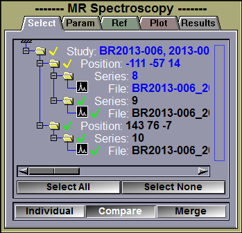
This interface tab enable you to select the datasets you want to analyze.
|
||
|
|
|
|
|
Selection Window |
The selection window let you select datasets by clicking on them or select a group of datasets by dragging a selection box, or clicking on the icon of an element higher in the hierarchy. Selected items will have a green check-mark. If you select some but not all the elements in a group, it's icon will have a yellow check-mark. Alternatively, you can select datasets directly by clicking on the highlighted voxels in the image window.
Note:
|
|
|
Select All / None |
These buttons let you select all the datasets or none of the datasets.
|
|
|
Individual |
If more than one datasets are selected, you have 3 options: You can see the plots of each datasets in an individual window, you can compare the selected datasets plots in the same window, or you can merge the selected datasets to try to improve the signal/noise of the data.
|
|
|
Compare |
||
|
Merge |
|
|
|
|
In this interface tab you can change the processing applied to the data of the dataset.
|
||
|
|
|
|
|
Apodization |
The choices are "Off", "Exponential" or "Linear". For "Exponential", the apodization is compute with: exp(-fact*x) (with 0<=x<=nb of data points) For "Linear", the apodizatrion is compute value decreasing linearly from 1 to 0 in a range of x in the middle of the nb of data points. values inferior to the range are clamped to 1, superior to the range to 0. The range is: "nb of data points / fact" with fact being between 1 and 20.
|
|
|
Zero Filling |
The choices are "Off" or "On". You select the total number of data points your dataset will have. All data points in excess to the original number of data points will be set to zero. The choices are power of 2 from 1024 to 16384
Note
|
|
|
Phase Correction |
Not yet implemented
|
|
|
Baseline |
The choices are "Off", "Power" or "Fourier".
For Power and Fourier, you then select how many terms the series will have: Power: y = A0 + A1 * x + A2 * x2 + A3 * x3 + ... + An * xn Fourier: y = A0 + A1a * cos(1πx/l) + A1b * sin(1πx/l) + ... + Ana * cos(nπx/l) + Anb * sin(nπx/l)
|
|
|
Data Filtering |
The choices are "Off", "Mean" or "Gaussian". You then specify the kernel's width (in % of the total number of data points).
Note
|
|
|
Peak Fitting |
The choices are "Off", "Lorentzian", "Gaussian" or "Voigt". For Voigt you need to select the ratio Lorentzian / Gaussian. If ratio = 0, then the peak are purely Lorentzian, for 1 they are purely Gaussian.
Note
|
|
|
T1/T2 Correction |
Not yet implemented
|
|
|
|
|
In this interface tab you can select which peak is the reference peak. The peak table give the peak positions in ppm, but the actual FFT transform give us data in Hz. To reconcile both, and have an Hz to ppm conversion, we need to have a reference peak that we can localize in the FFT.
|
||
|
|
|
|
|
Reference Peak Info |
The name of the reference peak, along with its position in ppm come from the peak table.
|
|
Ref selection window |
In this window you can select which peak is the reference peak. The program will automatically assign the reference peak to the first peak (from the left) that is at least 1/2 the height of the maximum peak. If this assumption is wrong, you can change it simply by dragging a selection box on the correct peak.
|
|
Dataset |
If you have multiple dataset selected, you can change the color of the plot lines for each individual datasets. If the datasets are merge together, then you can adjust the color for the merged values.
|
|
Recompute |
Recompute the peak fitting with the new Hz to ppm scale. |
|
|
|
|
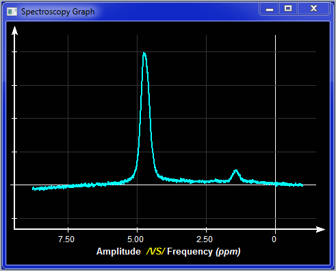
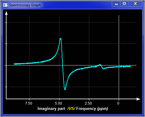
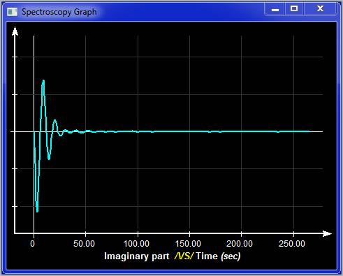
Frequency / Real |
You can display either the Frequency or the Time data, and either the real or imaginary component of the data. By default all frequency data is displayed in ppm. You can change this by pressing the "h" or "p" keys on the keyboard. They will toggle the scale between ppm and Hz.
|
|
|
Plot window |
This small window show you a preview of the plot window. You can zoom in a region of the graphic by dragging a selection region on the desired section of the graphic. The "Blow-Up" button is used to activate the plot window. You can also change the section of the curve that is displayed in the plot window by dragging a selection window in it. If you have a touch interface, you can use the 2 fingers to zoom on a specific region. The Blow-Up window also has a "zoom reset" button,
|
|
||||
|
Dataset |
If you have multiple dataset selected, you can change the color of the plot lines for each individual datasets. If the datasets are merge together, then you can adjust the color for the merged values.
|
|
|
Data |
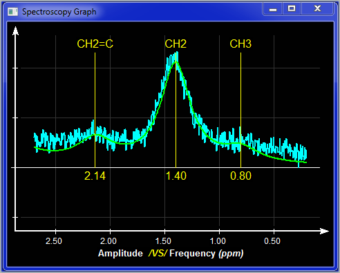
You can enable or disable the display of the raw data. Clicking on the "On" button a second time will enable the "On + Ri" mode where the residual "Ri" computed from the data minus the computed baseline and the computed peaks is displayed under the data curve. A third click will disable the display of the raw data ("Off"). You can also change the color used for this information in the plot window for each selected datasets.
|
|
|
Apodization |
In "Time" mode, you can display the apodization curve.
|
|
|
Filtered data |
in "Frequency" mode, you can display the filtered data.
|
|
|
Baseline |
in "Frequency" mode, you can display the value of the baseline.
|
|
|
Peaks |
in "Frequency" mode, you can display the computed peaks. You can either display a "Merge" curve of all the peaks, or, with a second click of the button, an "Individual" curve for each peak. |
|
|
|
|
|
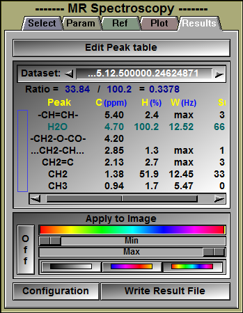
In this interface tab you can view and export the computation results.
|
|||
|
|
|
||
|
Edit Peak Table |
Clicking this button will open a peak edition window. In this window you will be able to add/delete peaks from the default peak table. The Edit Peak Table window is described in more detail further down.
|
||
|
Peak Results |
For each selected datasets, you can see the results from the peak fitting computation.
For each enabled peak in the peak table, we will display: •The peak's name •The peak's center (in ppm) •The peak's height (in % of the maximum value) •The peak's width (in Hz) •The peak's surface
Note
Note
|
||
|
Apply to Image |
The result of the ratio computation can also be displayed as a color on the images.
|
||
|
Configuration |
Clicking this button will open a configuration window. In this menu you will be able to specify the content and form of the result files you can create from this mode. The configuration menu is described in more detail further down.
|
||
|
Write Result File |
Create a result file. The results can be either in standard ASCII text, or in a tabulated form compatible with Excel. You can set the default for this with the configuration menu, or changing the "save as type" parameter in the confirmation pop-up window. |
|
|
|
|
On |
Enable the peak. only enabled peaks will be considered when fitting the peaks to the curves.
|
|
Ref |
Select the "Reference" Peak. This peak is used to compute the Hz to ppm conversion.
|
|
Name |
name of the peak
|
|
Center |
Starting center value of the peak (in ppm)
|
|
T1 / T2 |
Optional T1 and T2 values for surface T1/T2 correction (not implemented at this time)
|
|
A / B |
Select if the peak surface will be used in the numerator and/or denominator of the computed ratio.
|
|
|
Move up or down. More the currently selected peak line to the top or bottom of the table, or 1 line up or down.
|
|
|
Edit. Place the currently selected peak line in edit mode. The Name, Center, T1 and T2 values can be entered from the keyboard.
|
|
|
Add. Add a new line at the bottom of the table. By default, the new line is created in Edit mode.
|
|
|
Delete. Delete the currently selected peak line.
|
|
Max peak width |
The maximum width that a peak can reach (in ppm). If a peak reach that maximum, the width in the result table will be "Max".
|
|
Max peak drift |
The amount of drift allowed for each peak (in ppm).
|
|
Spectro Peak Table |
Specify the name of the file where the peak information will be saved. This file will be a scrip file.
|
|
Apply |
Apply the new settings to the current session of sliceOmatic and close the configuration menu.
|
|
Apply & Save |
Apply the new settings to the current session of sliceOmatic, save these values in the sliceO_ini.scp file for the next sessions and close the configuration menu. A description of that file is given in "The SliceO_ini.scp File" in the installation section.
|
|
Cancel |
Discard all changes and close the configuration menu |
|
|
|
|
Absolute/Relative |
The peaks heights and surfaces can be compute either from relative values (all curve heights are normalized by the highest peak) or absolute. If you are computing the ration between peaks, then the relative value will be O.K. But if you want to compare different acquisitions, then you need the "Absolute" values.
|
|
Result files can either be in plain ASCII text (compatible with notepad or any text editors) or in "DB file", a tabulated form, compatible with Excel or most spreadsheet programs.
|
|
|
You can have 3 optional headers in the files you created:
The Patient Info header
For each patient used in creating the file we will have (if the information is present in the image's header): •Patient Name •Patient ID •Patient sex •Date of Birth •Patient weight (Kg) •Patient height (m)
|
|
|
|
The Scanner Info header
For each scanner used in creating the file we will have (if the information is present in the image's header): •Modality •Manufacturer •Model
|
|
|
The Dataset Info header
For each dataset used in creating the file we will have (if the information is present in the dataset header): •Dataset Name •Acquisition matrix •Voxel position •Voxel dimensions •Nucleus •Transmitter Frequency (in MHz) •Number of data points (per columns) •Number of data points (per rows) •Field Strength (in Tesla) •Sequence Name •TR (in ms) •TE (in ms) •TI (in ms) •Number of averages
|
|
Saved Measures |
You can select which of the available measures you want to save in your result files.
|
|
Float Fraction |
You can specify whether you want the fractions in your floating point values to be delimited by a dot (".") (example:12.34) or a comma (",") (example: 12,34). By default it is the dot.
|
|
Cell Delimiter |
You can specify the character you want to use to mark the end of a cell in your spreadsheet result files. By default it is the "tab" character.
|
|
Cell Filler |
You can specify what should be placed in cells that have no values. For example, in a result file for multiple frames, if a TAG is not present in all the frames, then in some cells we will not have surfaces and volumes for it.
|
|
Default Path |
You can specify the default path for the results files. There is only one "default path" parameter in sliceOmatic, so by default, this value is set to the path of the last file read or written.
|
|
Default Name |
You can set a default name for your result files.
|
|
Cancel |
Close the configuration menu without saving any of the changes you just made.
|
|
Accept Changes |
Accept the changes you made and close the configuration menu. Please note that these changes only affect the current invocation of sliceOmatic. If you want to save the changes for future invocations of the program, you need to use the "Script Save As..." option of the File menu. |
From the Display Area
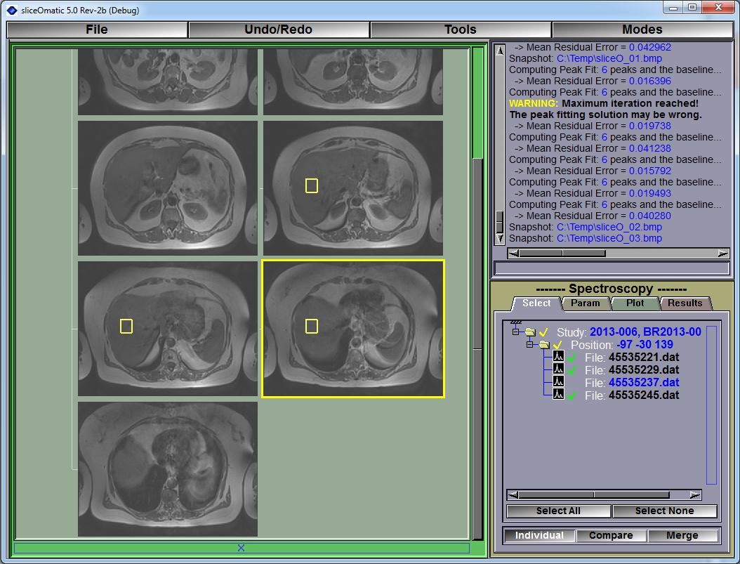 You can change the dataset selection by clicking on the corresponding region from the display area. The selected dataset voxels will be displayed in yellow, while the others will be in red.
Technical Note:
A typical spectroscopy dataset contain the UID of the images that are associated with it. When I first load these datasets, I locate all the matching images, then I use the UID of the Frame of Reference (FoR) of these images to locate all the images having the same FoR UID. For each of these images, if they intersect the volume of the spectroscopy voxel, I display the voxel's outline either in red or yellow.
From the Keyboard
The following keyboard key can be used while in this module:
|
|
|
|
|
|
Key |
Function |
|
|
|
|
|
|
"f" or "t" |
Toggle between the "Time" and "Frequency" modes in the plot window |
|
|
"r" or "i" |
Toggle between the "Real" and "Imaginary" modes in the plot window |
|
|
"h" or "p" |
Toggle between the "Hz" and "ppm" scale for the "Frequency" plots |
|
|
"b" |
By default, the baseline is compute along with the peaks when doing the Gauss-Newton least square iteration. This key will toggle a mode where the baseline is compute independently. |
|
|
"w" |
By default peak height and surface are compute relative to the highest peak in the data. Pressing "w" toggle this on or off. If "off" then the height and surface are compute directly from the values in the data. |
From the Command Line
System Variables defined in this library:
|
|
$SPECTRO_APODIZATION_FLAG |
(U16) |
Apodization flag: 0=off, 1=exponential, 2=linear (Default = 0) |
|
|
$SPECTRO_APODIZATION_FACT |
(F32) |
Apodization factor: Between 1.0 and 20.0 (Default = 10.0) |
|
|
$SPECTRO_BASELINE_FLAG |
(U16) |
Baseline flag: 0=off, 1=Power series, 2=Fourier series (Default = 1) |
|
|
$SPECTRO_BASELINE_FACT |
(U8) |
Baseline factor: Number of terms in the series (Default = 2) |
|
|
$SPECTRO_FILTER_FLAG |
(U16) |
Filter Flag: 0=off, 1=Mean, 2=Gaussian (Default = 1) |
|
|
$SPECTRO_FILTER_WIDTH |
(F32) |
Filter Width: Width of the filter's kernel in % of the number of data points (Default = 0.5) |
|
|
$SPECTRO_PEAK_FLAG |
(U16) |
Peak Fitting flag: 0=off, 1=Lorentzian, 2-Gaussian, 3=Voigt (Default = 1) |
|
|
$SPECTRO_PEAK_MIX |
(F32) |
Peak Fitting Mix (for Voigt only): between 0.0 (purely Lorentzian) and 1.0 (purely Gaussian) (Default = 0.5) |
|
|
$SPECTRO_PEAK_DRIFT |
(F32) |
Peak Drift: Maximum drift allow when fitting the peaks (in ppm) (Default = 0.1) |
|
|
$SPECTRO_PEAK_WIDTH |
(F32) |
Peak Width: Maximum width allow for the peaks when fitting (in ppm) (Default = 0.2) |
|
|
$SPECTRO_TABLE_PATH |
(S) |
Default path to the peak table definition script (Default = $DEFAULT_INSTALL_PATH\Spectro_Table.scp) |
|
|
$SPECTRO_WATER_SHIFT |
(F32) |
Default position of the water peak (in ppm) (to compute Hz to ppm scale) (Default = 4.7) |
|
|
$SPECTRO_ZERO_FILL_FLAG |
(U16) |
Zero Filling Flag: 0=off, 1=on (Default = 0) |
|
|
$SPECTRO_ZERO_FILL_FACT |
(I32) |
Zero Filling Factor: total number of data points (power of 2 from 1024 to 16384 (Default = 4096) |
|
|
$SPECTRO_MODE_RELATIVE |
(U16) |
Peak Height and Surface are relative to highest dataset value or absolute |
Commands recognized in this library:
Spectro: Mode (image|real|time|freq|ppm|hertz|baseline)
Set the current spectroscopy plot display mode:
|
|
Real |
The plot display the real component of the dataset |
|
|
Imaginary |
The plot display the imaginary component of the dataset |
|
|
Time |
The plot display the acquisition as function of time |
|
|
Frequency |
The plot display the acquisition as function of frequency |
|
|
ppm |
The frequency plot is labelled in ppm |
|
|
Hertz |
The frequency plot is labelled in Hertz |
|
|
Baseline |
|
Spectro: Mode (relative|absolute)
Set the current spectroscopy peak computation mode.
Spectro: Enable t_measure (on|off|toggle)
Enable or disable a measurement using a template. The template must match the measurement's name:
The available measurements are:
|
|
Name |
The peaks name (one value for each peak) |
|
|
Center |
The peaks center (in ppm) (one value for each peak) |
|
|
Height |
The peak height (in % of the maximum value) (one value for each peak) |
|
|
Width |
The peak width (in Hz) (one value for each peak) |
|
|
Surface |
The peak surface (no units) (one value for each peak) |
|
|
Ratio |
The ratio of the peaks surfaces selected for the numerator over the peaks surfaces selected for the denominator. (one per dataset). |
|
|
|
Spectro: type (text|db)
Set the default mode of the spectroscopy result file.
Spectro: name string
Set the default name of the spectroscopy result file.
Spectro: write [text|db] file_name
Write the results of the spectroscopy computation to the file "file_name" either in "db" or "text" form.
Spectro: table reset
Clear the spectroscopy peak table.
Spectro: table name
Create a new entry spectroscopy peak table. This new peak will be called "name".
Spectro: table name center value
Set the center value for the peak named "name" to the value "value" in the spectroscopy peak table.
Spectro: table name T1 value
Set the T1 value for the peak named "name" to the value "value" in the spectroscopy peak table.
Spectro: table name T2 value
Set the T2 value for the peak named "name" to the value "value" in the spectroscopy peak table.
Spectro: table name enable (on|off)
Enable or disable the peak named "name" in the spectroscopy peak table.
Spectro: table name numerator (on|off)
Add the surface peak named "name" in the spectroscopy peak table to the numerator in the ratio computation.
Spectro: table name denominator (on|off)
Add the surface peak named "name" in the spectroscopy peak table to the denominator in the ratio computation.
Spectro: param apo_flag (off|exp|linear)
Set the apodization mode.
Spectro: param apo_fact value
Set the apodization factor (float value).
Spectro: param zero_flag (off|exp|linear)
Set the zero filling mode.
Spectro: param zero_fact value
Set the zero filling factor.
Spectro: param phase_flag (off|zero|linear)
Set the phase correction mode. (currently disabled)
Spectro: param base_flag (off|power|Fourier)
Set the baseline correction mode.
Spectro: param base_fact value
Set the number of terms in the baseline correction series (integer value).
Spectro: param filter_flag (off|mean|Gaus)
Set the curve filter mode.
Spectro: param filter_fact value
Set the width of the filter kernel (floating point value).
Spectro: param peak_flag (off|Lorentz|Gaus|Voigt)
Set the peak shape.
Spectro: param peak_drift value
Set the maximum peak drift (floating point value, in ppm).
Spectro: param peak_width value
Set the maximum peak width (floating point value, in ppm).
Spectro: param peak_fact value
Set the voigt mix parameter value (floating point value).
Spectro: param T1T2_flag (on|press|steam)
Set the T1/T2 correction parameter (currently disabled).
Spectro: compute
Force a re-computation of the curves.
