This tool will compute an FFT (Fast Fourier Transform) of the frames and provide information on the frequency distribution of the frame's content.
The intent here is to provide a numerical value that is related to the presence of noise in the images.
The interface of this tool also allow you to visualize the real and imaginary part of the FFT of the frames as well as numerical values derived from the FFT.
|
|
|
|
|
|
|
|
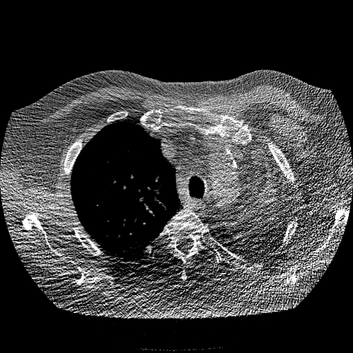
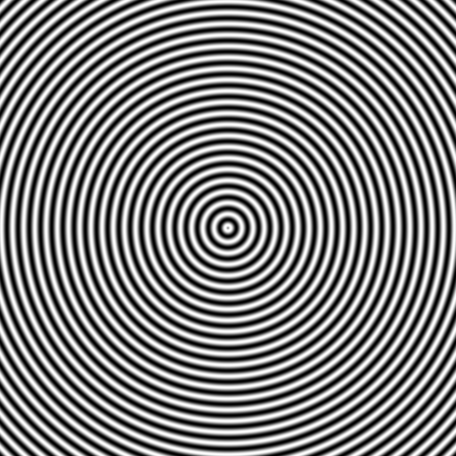
Normal CT image |
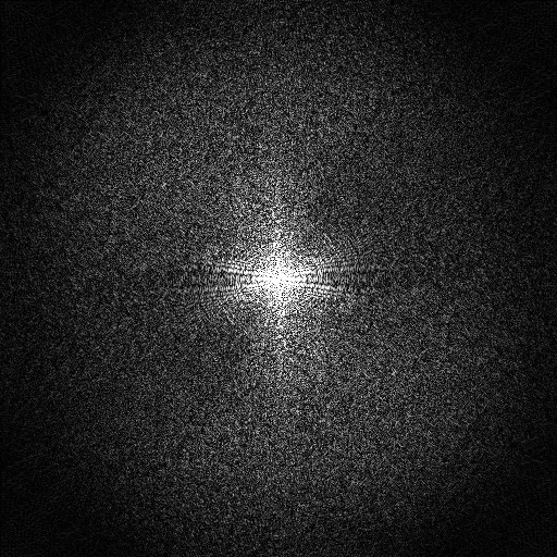
FFT of Normal CT image |
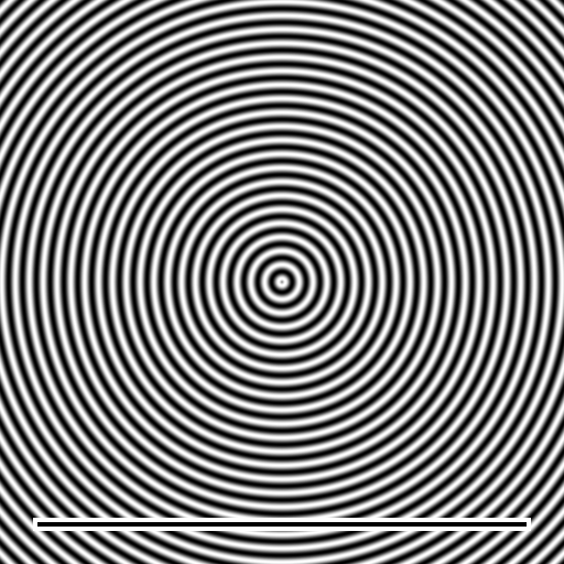
Noisy CT image |
FFT of Noisy CT image |
|
|
|
|
||
|
|
|
|
||


|
|
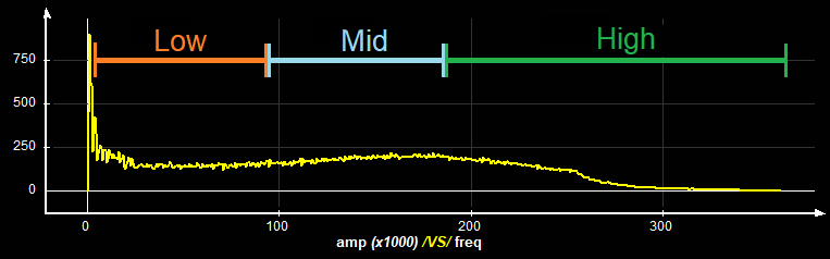
The numerical values are computed from the FFT transform of the image. The FFT transform the image from the spatial domain to the frequency domain. The lower frequency are at the center of the FFT and the higher frequency are on the borders. For each pixel of the FFT the tool compute amplitude of the FFT (square root of the square of the real and imaginary parts) and it's distance from the center. These values can be seen in the graph associated with each image. The amplitudes are then summed according to their distance from the center: In the first quarter of the distance we have the "Low" frequency, the second quarter, the "Mid" frequencies, and from half the distance to the border, the high frequency. The program also compute the ratio high frequency over low frequency to provide an index that reflect the "noisiness" of the image.
These 4 values (High/Low ratio, Low Freq. Mid Freq. High Freq.) are available to export in the Result 2D tool under the heading "Noise FFT".
|
|
Note:
|
|
|


From the Graphic Interface
|
|
|
|
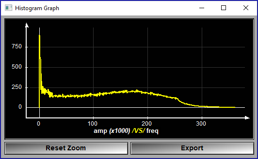
Frequency graph
|
This graph show the repartition of the FFT values as a function of their distance from the center of the FFT for the current frame. The "Blow" button open a window containing the same data. A first click open a normal window, a second click make it "top most" to prevent it from disappearing behind the sliceOmatic window.
|
|
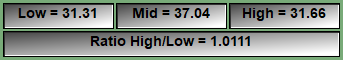
Low/Mid/High
|
The values for the "Low", "Mid" and "High" frequency as a % of the total are displayed for the current frame.
|
|
Ratio High/Low
|
The ration of High frequency over Low frequency. |
Display FFT
|
You can use these buttons to display the real or imaginary components of the FFT for all the frames. What is displayed is not directly the FFT values, but: ln( (ABS(FFT) + 1.0 ) * 100 |

From the Display Area
There is no Display Area interaction specific to this tool.
From the Keyboard
There is no keyboard interface specific to this tool.
From the Command Line
There is no command line or variables associated with this tool.