In this mode, you can use an AI to segment your 2D images, or if you want, you can train an AI on your previously segmented images.
This module work with individual images to automatically compute their associated TAG values. The images can be part of a 3D volume, but the 3D information is not used by the AI, each image is treated independently.
Note:
|
|
|

From the Graphic Interface
|
|
|
|
|
||
|
|
The main "AI with Python" interface has 3 tabs: Train, Test and Predict. Each of theses has a "Config" button that will open the configuration menu, and one (or more) "Compute" button that will open the appropriate page. |
||||
The Configuration Menu
Each of the 3 main pages of the "AI Python" interface has a "Config" button. This will open the configuration menu. Depending on the main pages you are in, the configuration menu will have between 3 and 8 sub-pages. For training, you need access to all the pages, for "Predict", you only need 3.
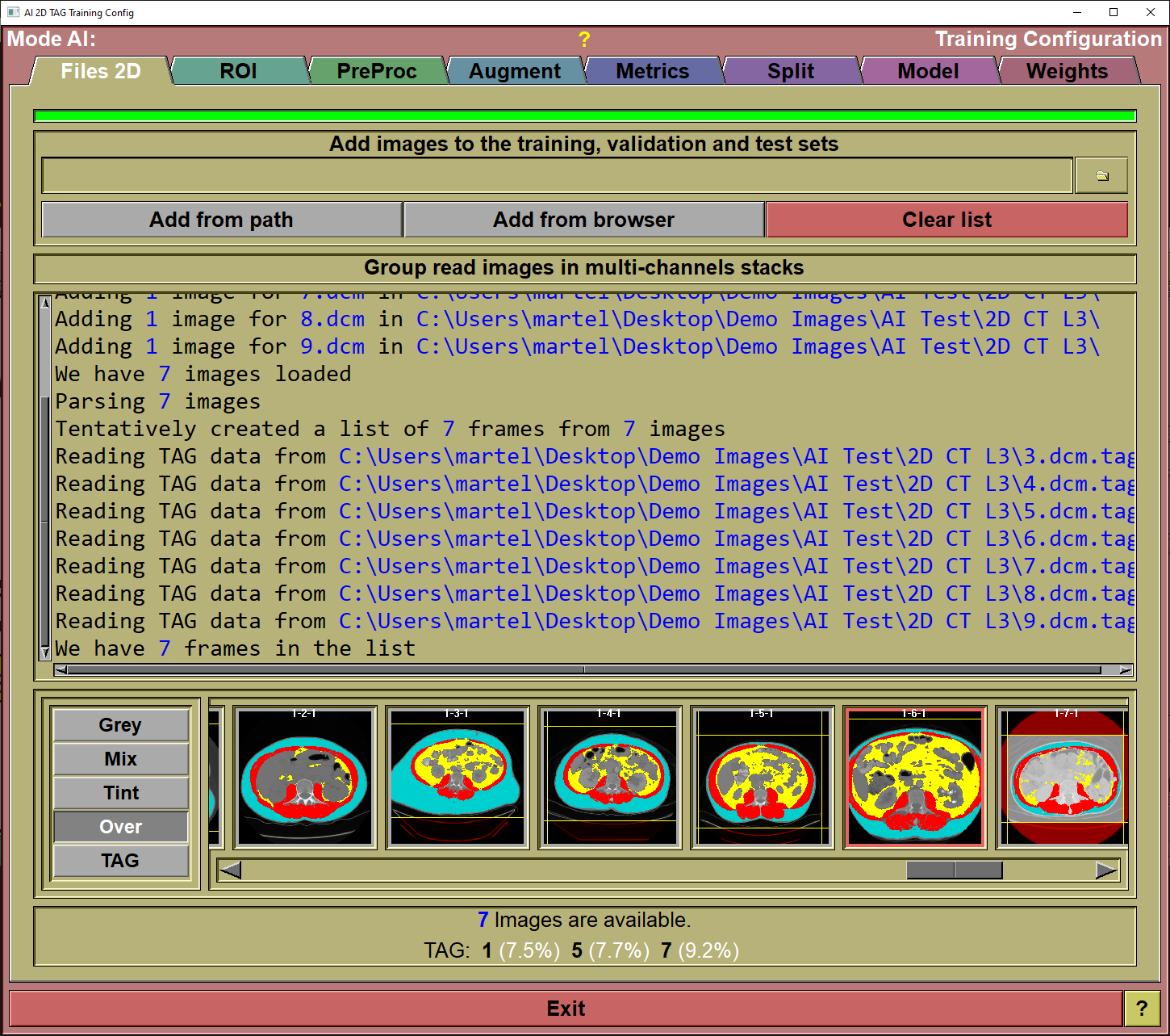
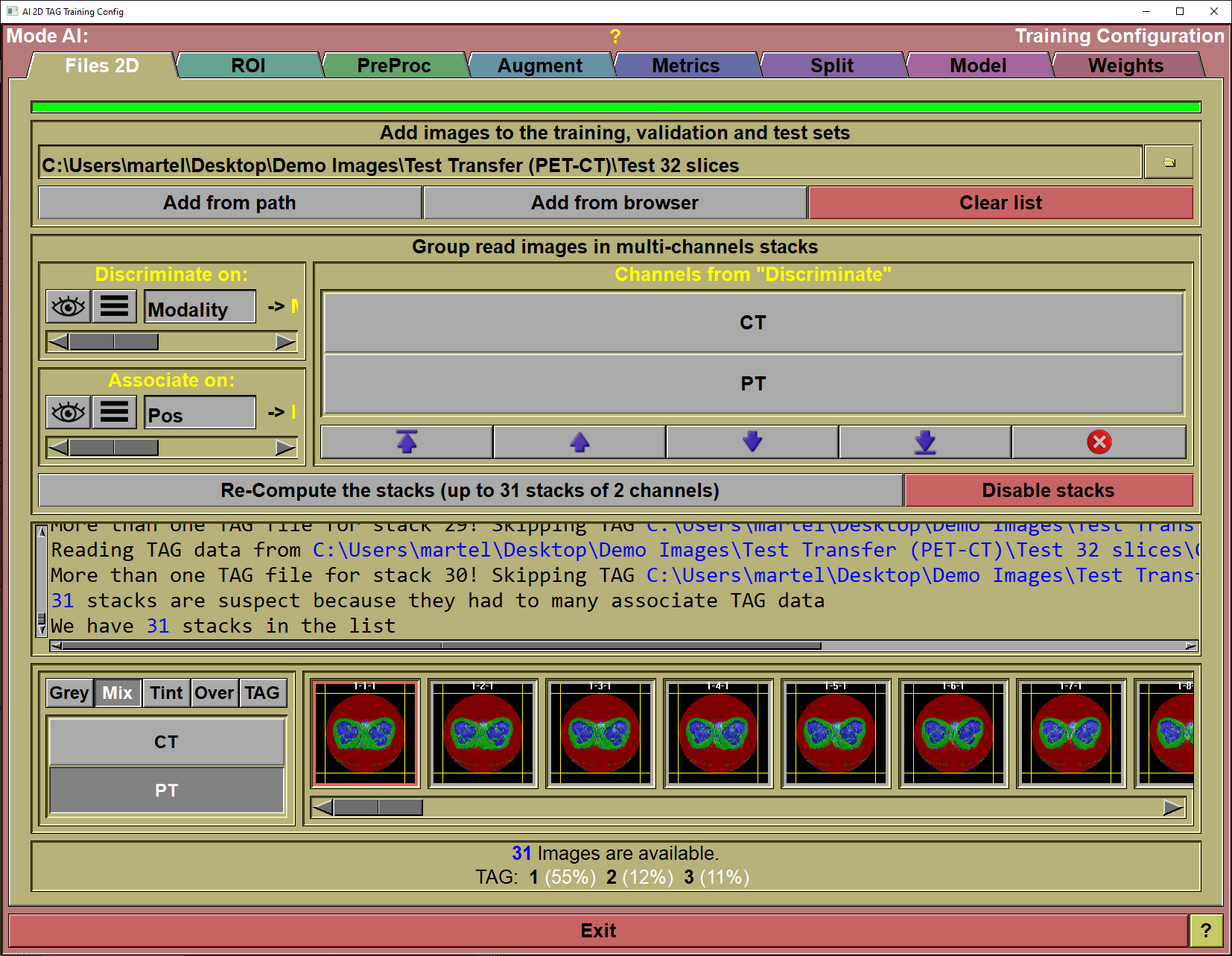
The config "File" page
This page is used to specify the images that will be used either for training or testing your AI.
|
|
|
Progress bar |
Show the progress of the program when parsing directories
|
Add slices |
Files can be added to this list in 3 different ways:
Simply drag&drop a directory on the interface. The program will recursively parse this directory and all its sub-directories. Each directories that contain segmented images will be add as a separate line in the interface or use the "From Path" or "From Browser" options.
|
From Path |
You can achieve the same results by specifying the directory in the input line and clicking the "Add from path" button.
|
From Browser |
You can add files with the "Medi Browser" interface.
|
Clear List |
Clear the list.
|
Multi-Channels
|
You can expand this section if you want to create stacks of multi-channel images. This is useful for modalities such as DIXON MR, CT/PET, MR/PET... When you have multiple images for the same slice and want to use all of them in the training.
|
Text Feedback |
When reading files or creating multi-channel stacks, the program give a feedback of what it is doing here.
|
Files preview
|
A preview of all the selected files is available.
|
Files status |
Show the number of images or stacks loaded in the AI. Also, the different TAGs found in these images (along with their prevalence) will be displayed.
|
Exit |
Exit the configuration interface.
|
Help |
Display this web page |
By default, the section "Group read images in multi-channels stack" is collapsed. But by dragging the separators you can expand it. You then have the possibility of having multiple images associated together. This can be used to analyze MR DIXON/IDEAL images or even PET/CT images. Instead of working with single frames, the AI will work with "stack" of images. The images in the stack do not need to be of the same field of view or resolution, they don't even need to be aligned. They do need to be coplanar and have an overlap though.
If you do activate the "Multi-channels stacks", then the "Preview" section will have an additional group of buttons to let you see the different channels in the stack.
|
|
|
Discriminate on |
The value of this parameter decides in which channel the frames from each file will go.
You can select the parameter from a pull-down list using the
The parameter can be a DICOM tag or one of the accepted key-words: "path", "name", "ext", "suffix", "time", org", "pos", for", study", "series", "image", acquisition" or "modality".
DICOM tag are the form (xxxx,yyyy) where "xxxx" is the DICOM group and "yyyy" is the DICOM tag.
In some cases, you may want to discriminate on a specific key-word inside a DICOM tag. You can do this by enable the "Key Words" button, typing the keywords (separated by ";") and pressing "Enter" to activate the filter. You need one key-word for each channels.
There is a more detailed description of the discriminate/associate parameters in the Class Mixer page.
|
Associate on |
The value of this tag will be used to match frames across channels.
You can select the parameter from a pull-down list using the
The parameter can be a DICOM tag or one of the accepted key-words: "path", "name", "ext", "suffix", "time", org", "pos", for", study", "series", "image", acquisition" or "modality".
DICOM tag are the form (xxxx,yyyy) where "xxxx" is the DICOM group and "yyyy" is the DICOM tag.
In some cases, you may want to associate frames on a specific key-word inside a DICOM tag. You can do this by enable the "Key Words" button, typing the keywords (separated by ";") and pressing "Enter" to activate the filter. You need one key-word for each association.
There is a more detailed description of the discriminate/associate parameters in the Class Mixer page.
|
Channel from discriminate |
A list of the channels found in your images from the "Discriminate on" parameter is displayed here. You can change the order of the channels or even remove channels that you do not want to use in the AI.
|
Channel from weights |
If you have loaded weights that have been computed from stacks, you can see the channels that where used during the training of these weights. You can also see if the channels where swapped or if the training was done with some channels deactivated.
|
Re-compute the stacks |
Once you have set the "Discriminate on", "Associate on" and set the channels order, you can re-compute the stacks with these parameters.
|
Disable stacks |
If you do not what to use stacks, click on this button to revert to individual frames.
|
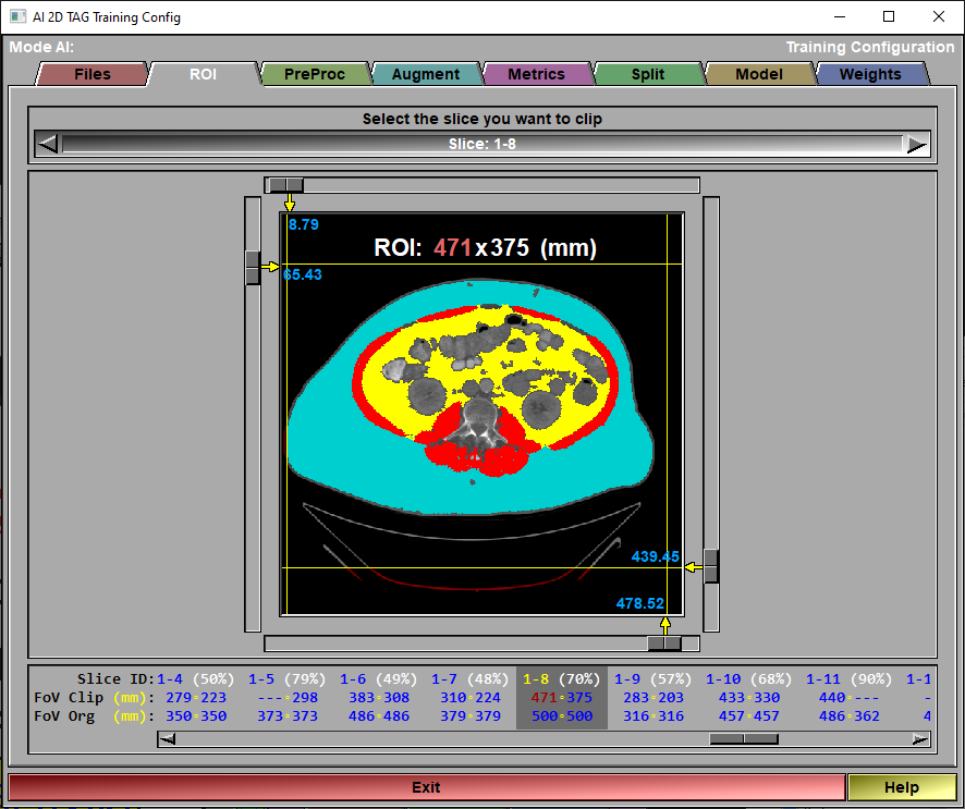
The config "ROI" page
This page is used to limit the surface of each slices used in training or testing. The currently displayed image can be selected from the selection tool at the top or from the list of frames at the bottom. We display in red the values that are currently the maximum for each X and Y dimensions. That way, it is easy to identify the frames that would benefit from being clipped.
|
|
|
Slice selection |
You can select the slice you want to clip from this list. - You can also use the mouse scroll wheel when the cursor is not over one of the clip sliders. - You can also click on the desired slice in the "Clip status" region.
|
Clip planes |
You can move the 4 clip planes used to define the ROI for each slice.
|
Clip status |
The status for each slice is composed of 3 lines: •The slice number (directory - slice) along with the ratio of the ROI over the complete slice. •The clipped FoV. Or the dimensions of the ROI defined by the clip planes. The highest FoV value will be displayed in red. •The original FoV of the slice. |
|
|
|
Exit |
Exit the configuration interface.
|
Help |
Display this web page. |
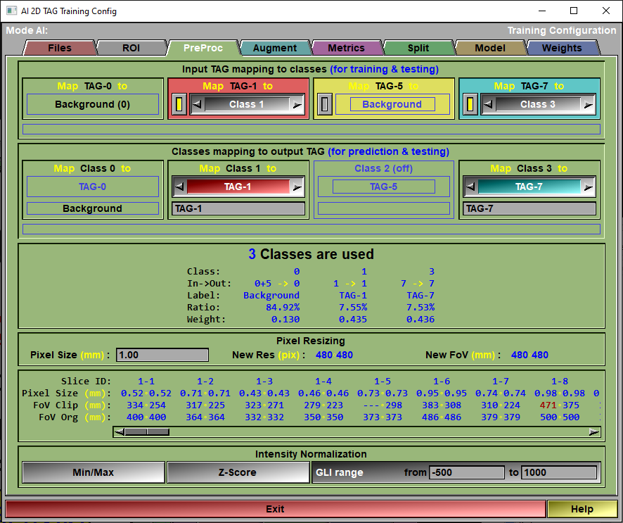
The config "Preproc" page
This page is used to control any pre-processing that need to be applied to the images. You also use it to select the classes used in your AI.
Note:
|
|
|
|
|
|
Input TAG mapping
|
In this section, there is one box for each TAG present in the selected images. The title of the box (ex: "Map TAG-1 to") let you know what TAG is being mapped. Each of these can be mapped to a "Class" for the AI.
At first, there is as many classes as there are TAGs in the selected images. But since multiple TAGs can be mapped to the save class, some of the classes can be disabled if no TAG mapped to them. So, if there is a TAG in the images you do not want to use in the AI, just map it to the background. If in sliceO you identified different muscles with different TAGs, but you do not need the AI to differentiate these muscles, map all the muscle TAGs to the same class.
If you want to completely disregard a TAG value, map it to the "Background". This can also be done by simply clicking the button on the left side of the TAG's interface.
This mapping is only used for training and testing. When predicting, only the grey values of the image is used.
|
Class mapping
|
Each classes used in the AI can be mapped to a TAG value. So, for example, if you map "Class 1" to the "TAG-1", when predicting the segmentation of an image, the tissue associated to Class 1 will be tagged in sliceO using TAG-1. You can also assign a label to that TAG. That label will be used in the AI reports and, if you use the AI to segment images, assigned to the corresponding TAG in the sliceO's interface.
This mapping is only used for predicting and testing.
|
Mapping status |
An overview of the current classes and how they are mapped, along with their label and the ratio of pixels (with the associated weights) is presented here. The "Weight" values are used in the different "Weighted" metrics.
|
Pixel resizing |
Before training, testing or predicting on the slices, they will all be re-sized to the desired pixel size. So the pixel size you chose will affect the precision of your prediction. You want a smaller pixel for more precise results. On the other hand, a smaller pixel size will result in bigger images (higher resolution) so the training will take longer.
There is no reason to have a pixel size smaller than the smallest original pixel size (see "Resizing status").
Once you select a pixel size, the program will use it to divide the biggest FoV (in both X or Y) from all the loaded images to find the resolution that will be used in the training. This resolution must be a multiple of 16 for the U-Net model to work. The FoV of the training dataset will then be the pixel size multiplied by new resolution.
If you want to increase the training speed, you may want to reduce the FoV of the biggest image using the ROI interface. The biggest FoV value will be displayed in red in the Resizing status region.
|
Resizing status |
For each slice we will have 3 lines of information: - The slice number (dir - slice). - The original pixel size. - The clipped FoV (maximum values are displayed in red). - The original FoV.
|
Intensity Normalization |
The AI expect floating point pixels values between -1 and 1. While medical images use integer values. So, we need to "normalize" the pixel values.
You have 3 choices: "Min/Max", "Z-Score" or "GLI range".
The "Min/Max" normalization will normalize the GLI values so that the minimum value found in an image will be -1 and the maximum will be 1.
The "Z-Score" normalization will normalize the GLI values so that the mean value of an image will be at 0 and and the standard deviation is 1. The idea is that all the values within 1 standard deviation of the mean will be between -1 and 1.
The "GLI range" is mainly used for CT images. All HU values under the minimum will be assigned a value of -1, and all HU greater than the maximum will be assigned a value of +1 in the normalized images. All HU values in-between will be linearly mapped between -1 and 1.
|
Exit |
Exit the configuration interface.
|
Help |
Display this web page. |
Note:
|
|
|
Note:
|
|
|
Note:
|
|
|
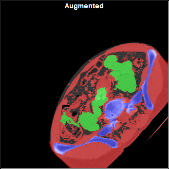
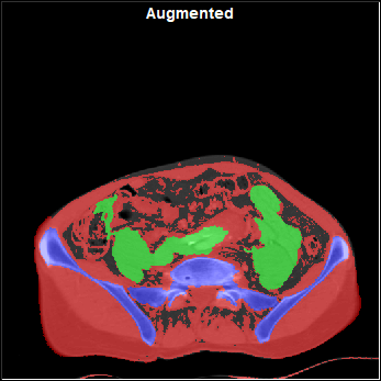
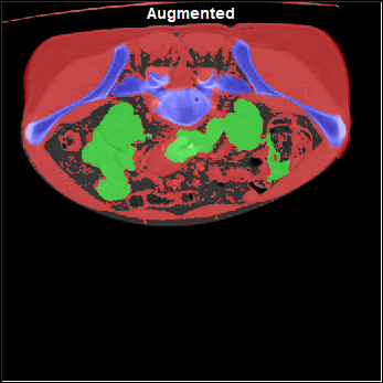
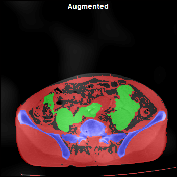
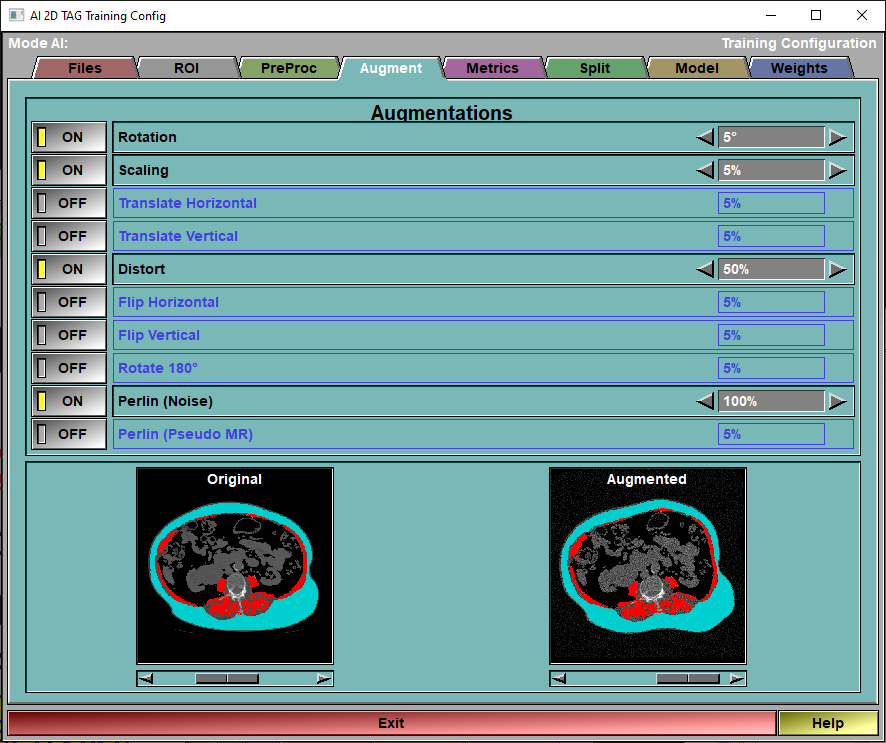
The config "Augment" page
This page enable you to select and control the different augmentations that are applied to the images before they are used for training. The augmentations will be applied to all the "training" images before each epoch. Only the "Training" images are augmented, the images reserved for validation and testing are never augmented.
|
|
|
|
|
|
|
|
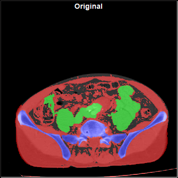
Original Image |
Rotated |
Scaled |
Translated |

|
|
|
|
|
|
|
|
Distorted |
Flipped |
With Noise |
With "Pseudo MR" |

|
|
|
||||||||||||||||||
Augmentations |
You can enable/disable the different augmentations, and specify the intensity of each of these from this interface. You have access to 9 augmentations. Each of these is controlled by a selected value "val":
|
||||||||||||||||||
Demo Original |
The slider under the image is used to change the demo frame. All the images used for training are available.
|
||||||||||||||||||
Demo Augmented |
The slider under the image is used to show the range of augmentation.
In normal training images, each time an image is augmented, a random value between -1 to +1 is assigned to each augmentation of each image.
In this demo however, we use the slider to show the range of possible augmentation. The slider simulate the random variable, with a range of -1 (complete left) to +1 (complete right).
|
||||||||||||||||||
Exit |
Exit the configuration interface.
|
||||||||||||||||||
Help |
Display this web page. |
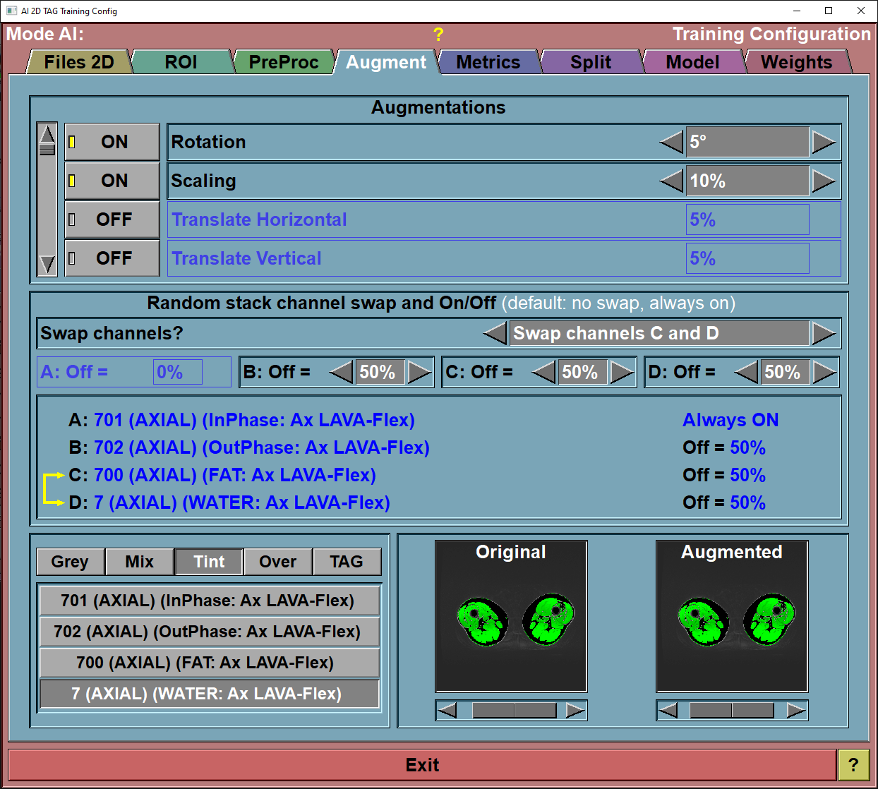
If you have created stacks in the "File 2D" config page, then you also have some augmentations that can be done inside the stacks. You can randomly swap channels (either all the channels or any pair of channels). You can also force some channels to "0" a certain portion of the time. This will enable you to use the computed weights that can be used with or without that channel being present in the prediction.
|
|
|
Swap channels |
|
Turn channels off |
|
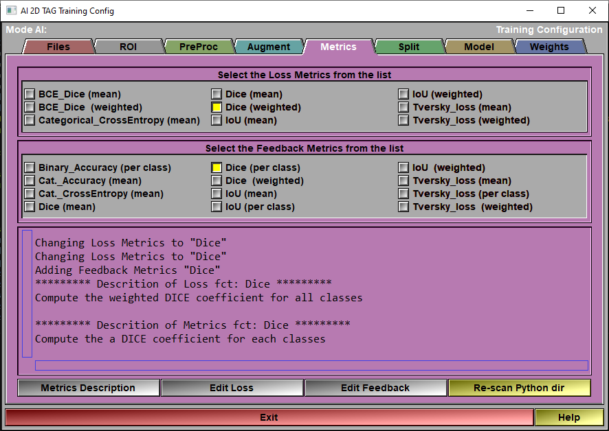
The config "Metrics" page
When you train the AI, 2 sets of "metrics" are used: The Loss Metrics is the one used to compute the AI weights. The other group of metrics are just computed to give you an idea of what is going on. They are only there to provide you some feedback on the accuracy of the AI, they are optional and can be all off if you want.
At this time, you can only have 1 "Loss" metric when training your AI. You can however have as many "Feedback" metrics as you want.
These metrics will be reported back to you when you train your AI. They can also be used when you will select the weights you want to save for your AI. During training you will be presented with 2 graphs: One for the training and validation loss, and one for the training and validation values of the feedback metrics.
|
|
|
|
Loss Metrics |
Select one of the metrics as a "Loss" function to train the AI.
|
|
Feedback Metrics |
Select any metrics you want from this list to get additional information on the AI training progress.
|
|
Text Window |
This window reports on the metrics selections and the description of each metrics.
|
|
Description |
This will cause the description associated with each of the selected metrics to be displayed in the text window.
|
|
Edit Loss |
The different metrics are all Python files that you can edit if you want. You can also add your own metrics. Just follow the prescribed syntax and add the python file of your new metric in the Python directory. Then click the "re-scan dir" to cause sliceO to re-analyze the directory and add your metrics. The syntax will be described later at the end of this section. |
|
Edit Feedback |
|
|
Re-scan dir
|
|
|
Exit |
Exit the configuration interface.
|
Help |
Display this web page. |
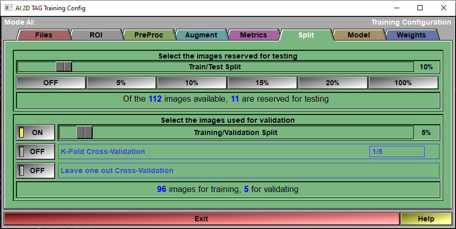
The config "Split" page
|
|
|
|
Testing |
A portion of the images you selected in the config "File" page can be reserved for testing.
|
|
Testing Status |
Report on the number of available images
|
|
Validation |
You have access to 3 validation methods: •Training/Validation Split. Probably the simplest, a part of the available images (those left after the images reserved for testing are removed) is reserved for validating the AI at each epoch. The same images are used for validation at each epoch. •K-Fold Cross-Validation. The available images are split in "n" groups using the ratio defined in the K-Fold interface. For example if the K-Fold is 1/5, then n=5. We do a complete training of all the epochs reserving the images of one of these groups validation. We then redo the complete training using another group for validation. We do this n times. After that, we assume that we have a good idea of the validation since by now all the images have been used for that, we do a last training without any validation. In the "Train Save" page, the graphs will show the mean value of the n+1 pass for training metrics and the n pass with validation for validation metrics. •Leave one out Cross-Validation. This is the extreme case of K-Fold where n is equal to the number of images.
|
|
Validation Status |
Report the number of images that will be used for training and for validation.
|
|
Exit |
Exit the configuration interface.
|
Help |
Display this web page. |
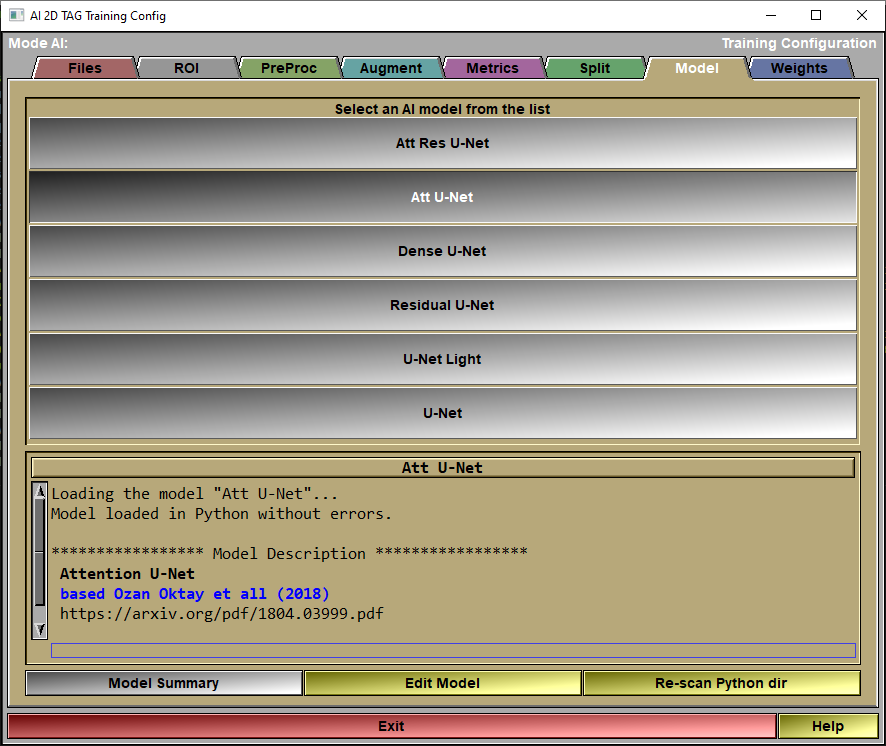
The config "Model" page
In this page, you will select the model you want to use for the AI.
|
|
|
|
Model List |
Select a model from the list.
|
|
Model Feedback |
Information on the selected model will be displayed here.
|
Model Summary |
Call the Keras function "Summary" for the selected model.
|
Edit Model |
The different models are all Python files that you can edit if you want. You can also add your own models. Just follow the prescribed syntax and add the python file of your new model in the Python directory. Then click the "re-scan dir" to cause sliceO to re-analyze the directory and add your model. The syntax will be described later at the end of this section.
|
Re-scan Python dir
|
|
|
Exit |
Exit the configuration interface.
|
Help |
Display this web page. |
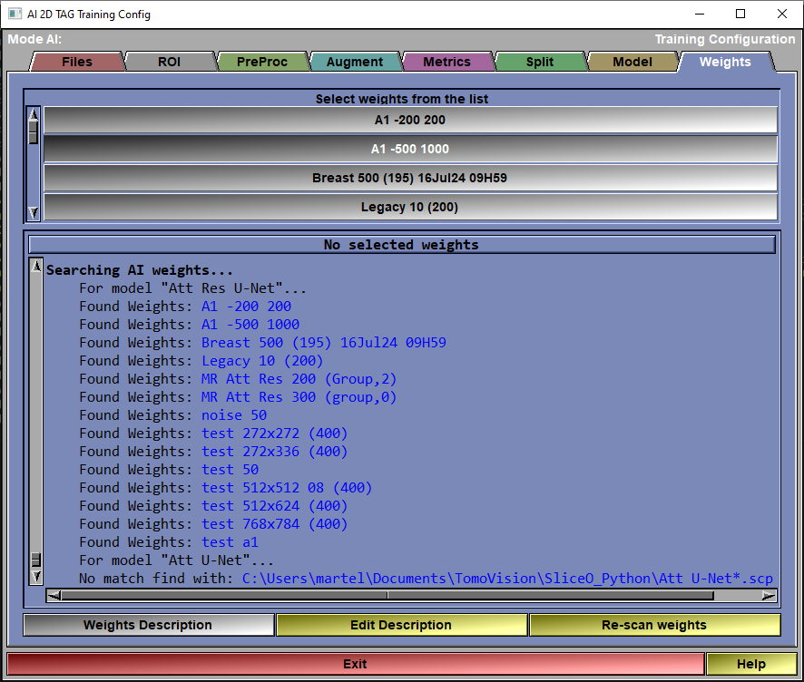
The config "Weights" page
|
|
|
|
Weight List |
This list will display all the available weights for the selected model. Select one of these from the list.
|
|
Weight Feedback |
Information on the selected weights will be displayed here.
|
Weight Description |
Cause the description of the weights to be displayed in the text window.
|
Edit Description |
The weight description is a text file associated with the weights. It has the same name as the weights but with the ".txt" extension. It can be edited with a simple text editor. If you click "Edit", this file will be opened in Notepad.
|
Re-Scan weights
|
Re-scan the directory if you have saved some new weights for this model. |
|
Exit |
Exit the configuration interface.
|
Help |
Display this web page. |
|
|
|
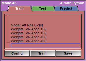
Text Feedback |
|
Config |
Open the Configuration window
|
Train
|
Open the "Train" Window. |
Save |
Open the "Save" Window.
|
Once you used the config pages to select the files you want to train on, and you selected the preprocessing steps, the augmentations, the validation split and the model you want to use, you are ready to start training your model to obtain the AI weights.
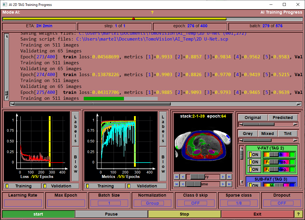
This is the page that will enable you to train the AI.
The only things that remain for you to select are the learning rate, the number of epochs and the batch size. After that, you click on "Train" and wait (and wait... and wait...) for the results!
Once started, the training will:
•Pre-load and normalize all the images used for training and validation in memory.
Then, for each step it will:
•Reset or pre-load the weights (if you selected to re-train existing weights).
Then, for each epoch it will:
•Reset and augment all images used for training.
•Make a scrambled list of the images used for training.
•Call the Keras function "train_on_batch" for the batches of training images (using the scrambled list).
•Call the Keras function "test_on_batch" for the batches of validation images.
•Report the results of this epoch and possibly save the current weights, the current metrics and a script associated with these to the "AI Temp" folder. We only save a total of 100 weights, so if you have more than 100 eopchs, we will only save weights each (nb_epoch/100) epochs.
The number of "steps" is dependant on the validation technique. A simple Train/Validation split us done in a single step. K-Fold and Leave-one-out cross validation require multiple steps.
Note:
|
|
|
Note:
|
|
|
Note:
|
|
|
|
|
|
|
Progress Bar |
Report on the training progression.
|
|
ETA |
Estimated time of completion (computed after each epoch).
|
|
Step Feedback |
Current step number.
|
|
Epoch Feedback |
Current Epoch number.
|
|
Batch Feedback |
Currently processed batch.
|
|
Text Feedback |
textual information about the training progression.
|
|
Loss Graphic |
A graphic showing the training and validation loss values as a function of the epochs.
|
|
Validation Graphic |
A graphic showing the training and validation values of all the selected feedback metrics
|
|
Progression Feedback
|
The content of this window is function of the "Display validation images" option you set in the "file\config" page, the "AI" tab. The choice are:•History: The program will save images of each of the validation slices when it save the training weights. You can then use this window to look at the validation results at the different training epochs. (Make sure you have enough space in your "Document" folder to contain a maximum of 100 copies of the validation images segmentations.) •Latest: You can see the validation results for the latest training epoch. •Off: This window will remain blank.
The window is separated in 2 sections:•On the left you see the validation images and you can use the controls to change the epoch (if you selected "history") or the displayed validation image. •On the right you can chose to see the true (original) segmentation values, the results of the training (predicted) of a mix of both. If you select both, the intensity of the TAG colors will be decrease if both the original and predicted values are the same. This highlight the errors (false negative and false positive) made by the AI. You can also select the color mode (Grey, Mixed, Tint, Over or Tag) controlling the mixing of the grey level values with the TAG colors. If you have enabled the multi channels stacks, you can select which of the channels are displayed as grey level images. After that you have 3 buttons and sliders per classes. For each class computed by the AI, you enable/disable and change the color of 3 group of pixels: •The pixels that have this TAG value in both the original and predicted images. •The pixels that have this TAG value in the predicted image only (False Positive) •The pixels that have this TAG value in the Original image only (False Negative)
|
|
Learning Rate |
The learning rate used in training the AI. the default value is 0.001
|
|
Max Epoch |
The number of epoch used for the training.
|
|
Batch Size |
The number of images used in each training and testing batches. If the AI failed because of a lack of GPU memory, you can decrease this value.
|
|
Normalization |
The AI need the values of the training dataset to be close to the range "-1" to "1". But a lot of the model's computations will cause the values to drift from this range. You can select to "Normalize" the data at each step of the model. You have the choice of 3 normalization modes: •Batch •Group •Instance
The "Normalization" value is placed in the system variable: "$AI_NORMALIZATION" and is accessible to the model. This is explained further down.
|
|
Class 0 skip |
You can ask the AI to disregard the class 0 (the background) in the loss computation. This will help the AI to converge toward classes that have a surface a lot smaller than the surface of the background. The trade-off is that you may have more false positive pixels since the AI has disregarded the background.
|
|
Sparse classes |
If a class is only present in a portion of the images used in training, the AI may find that it is easier to simply not predict any pixels of that class. It still get a perfect score for the slices where the class is absent.
The "Sparse classes" option prevent this in 2 ways:
a) It sort the images to keep the ones without any presence of the class in one group and only use a portion of these when computing the loss contribution of the class. You have the choice between •"0": The class does not contribute to the loss of any of the images where it is not present. •"1/16": Only 1/16 of the images without the class are used in the loss computation fro that class. •... •"1/2": Half the images without the class are used in the loss computation for that class. •"1": As many images without the class as they are images with the class will be used in the loss computation. •"all": All the images will be used in the loss computation. If the class is lost, we will rely on "b)" to save it.
b) If the program detect that the AI has dropped a class, it will rewind the training to the last saved epoch. It will also place the "Sparse class" parameter to "0" for a fixed ($AI_2D_SPARSE_SKIP) number of epochs. If we still lose the class during that interval, we will rewind further, and if that didn't work, we will consider the class lost.
|
|
Dropout |
A technique to help the training to converge is to "drop" a number of the computed weights at each step of the computation. A "dropout" of 0.3 for example will reset 30% of the weights to zero. This help prevent the training from converging toward a false local minima.
The "Dropout" value is placed in the system variable: "$AI_DROPOUT" and is accessible to the model. This is explained further down.
|
|
Start |
Start the training.
|
|
Pause/Resume |
You can pause and resume the training.
|
|
Stop |
Stop the training.
|
|
Exit |
Exit the "Training" interface.
|
|
Help |
Display this web page. |
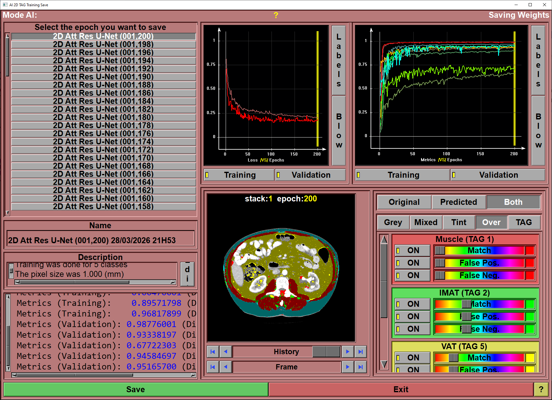
After having trained your AI, you want to save the weights you just computed.
When clicking "Save" 4 files will be transferd from the "AI Temp" folder to a sub-directory of the "Python Code" folder. This sub-folder will have the name of the model used for the training (ex: "U-Net", "Att Res U-Net"...). That sub-folder will contain 4 files, they will all have the name you selected but with different extensions:
•The Keras generated weights (with the extension ".data-00000-of-00001"). This file will be big (more than 100Mb).
•The Keras generated index (with the extension ".index"). This file has between 30Kb to 40Kb.
•A sliceOmatic script file containing the training parameters (with the extension ".scp").
•An ASCII "description" file (with the extension ".txt").
Note:
|
|
|
To help you select the optimal epoch for the weights, you have access to plots of the loss and feedback values along with their numerical values.
|
|
|
|
Epoch Selection |
Select the desired epoch from the list.
|
|
Name |
Name use for the saved weights. A default value is proposed, but you can change it as you which.
|
|
Description |
The description associated with the saved weights. Again, a default value is proposed, but you can edit this test to your liking.
|
|
Epoch Feedback |
Numerical values of the different metrics at the end of the selected epoch.
|
|
Loss Graphic |
Plot of the training and validation loss as a function of the epochs. The yellow vertical bar represent the selected epoch. You can also select the epoch to save by clicking at the desired location in the graphic window
|
|
Validation Graphic |
Plot of the training and validation feedback metrics as a function of the epochs. The yellow vertical bar represent the selected epoch. You can also select the epoch to save by clicking at the desired location in the graphic window
|
Validation Feedback |
The content of this window is function of the "Display validation images" option you set in the "file\config" page, the "AI" tab. The choice are:•History: The program will save images of each of the validation slices when it save the training weights. You can then use this window to look at the validation results at the different training epochs. (Make sure you have enough space in your "Document" folder to contain a maximum of 100 copies of the validation images segmentations.) •Latest: You can see the validation results for the latest training epoch. •Off: This window will remain blank.
The window is separated in 2 sections:•On the left you see the validation images and you can use the controls to change the epoch (if you selected "history") or the displayed validation image. •On the right you can chose to see the true (original) segmentation values, the results of the training (predicted) of a mix of both. If you select both, the intensity of the TAG colors will be decrease if both the original and predicted values are the same. This highlight the errors (false negative and false positive) made by the AI. You can also select the color mode (Grey, Mixed, Tint, Over or Tag) controlling the mixing of the grey level values with the TAG colors. If you have enabled the multi channels stacks, you can select which of the channels are displayed as grey level images. After that you have 3 buttons and sliders per classes. For each class computed by the AI, you enable/disable and change the color of 3 group of pixels: •The pixels that have this TAG value in both the original and predicted images. •The pixels that have this TAG value in the predicted image only (False Positive) •The pixels that have this TAG value in the Original image only (False Negative)
|
|
Save |
Save the selected weights to the model's sub-folder.
|
|
Exit |
Exit the "Save" interface.
|
|
Help |
Display this web page. |
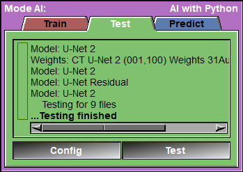
This page is used to test your AI against a reserved portion of the selected images.
The program will go through all the "test" images, and call the Keras "test_on_batch" function for each of them. It will report the different metrics for each images and once all the images are tested, compute the mean and standard deviation of each of the metrics.
These results will also be saved in a Excel compatible file in the AI_Temp directory.
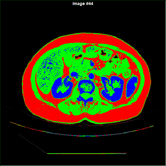
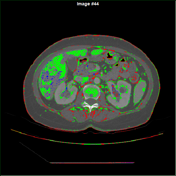
You will also be able to view each of the tested images. You can view the original segmentation, the predicted segmentation and a mix of both. in the "both" mode, the TAG that are un-correctly predicted will be full color, while the correct prediction will be darker. You also have control over the display options for the match, false positive and false negative values of each TAG.
|
|
|
|
|
|
|
|
Original segmentation |
Predicted segmentation |
Both in mode "Over" |
Both in mode "Grey" |


|
|
|
Text Feedback |
|
Config |
Open the Configuartion window
|
Test |
Open the "Test Progress" Window.
|
|
|
|
Progress Bar |
Show the progression of the testing
|
Text window |
Report on the metrics for each image and the mean values.
|
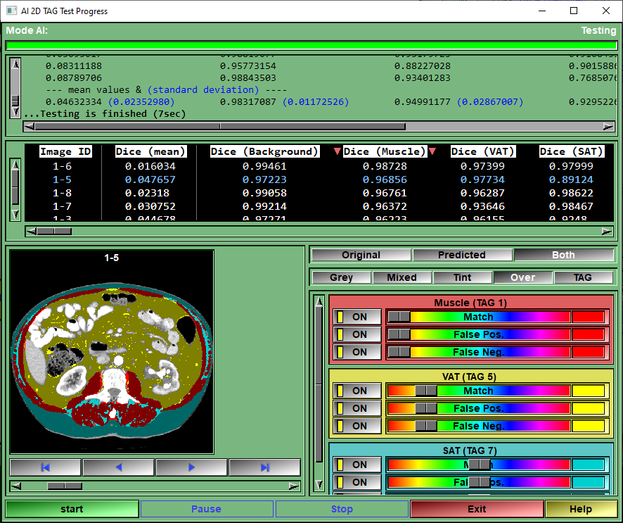
Results box
|
Once the testing is done, this box will display the numerical results of the different metrics.
The results can be sorted according to any of the presented columns. Just click on the column title to change the sort order.
The line matching the test volume selected for display will be highlighted in blue. You can select any of the test volumes for display by clicking on its line.
|
Test image |
Show the test images.
|
Image selection |
You can display any of the images used for testing. the arrow keys will advance to the first image, the previous image, the next image, the last image. You can also use the slider to select images. The images are sorted from the one with the worst to the best "Loss" metrics.
|
Source selection |
You can display either the original segmentation, the predicted segmentation, or a mix of both.
|
Display Mode |
This is the same controls as the "2D Color Scheme" tool in sliceOmatic. the "F1" to "F4" keys can also be used as shortcuts.
|
TAG Color |
For each TAG computed by the AI, you enable/disable and change the color of 3 group of pixels: •The pixels that have this TAG value in both the original and predicted images. •The pixels that have this TAG value in the predicted image only (False Positive) •The pixels that have this TAG value in the Original image only (False Negative)
|
Start |
Start the computation of the tests.
|
Pause/Resume |
Pause/resume the computation.
|
Stop |
Stop the computation.
|
Exit |
Exit this page.
|
Help |
Display this web page.
|
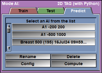
The Predict page
This is the page where the magic happens!
From the AI list, select the AI you want to use. Alternatively, you can use the Config page to select a model and its assciated weights.
Select the desired images in sliceOmatic and click on the "Compute" button.
Note:
|
|
|
|
|
|
AI Selection |
Select the desired AI from the list. This will automatically set the Model and the associated Weights.
|
Rename |
Rename the files associated with the selected AI (script, text and AI weights).
|
Delete |
Delete the files associated with the selected AI.
|
Config |
Open the Configuration window
|
Compute |
Open the "Predict Compute" Window.
|
The goal of the AI module is to compute the segmentation automatically. This is done here.
The prediction module is the one that compute the segmentation. The segmentation is computed from the selected weights chosen in the "Predict" tab (or from the "Config" menu). The training has been done at a specific pixel size and slice resolution. This (pixel size x resolution) give us the training ROI. If any of the loaded images in sliceO has a FoV larger than the training ROI, the prediction will only be computed on a portion of the slice. You can use the prediction interface to place the ROI where you want on the loaded image.
If the selected weights have been trained with multiple classes and you only want to get the prediction for one tissue, you can use the "TAG Lock" tool to protect the other tissues.
|
|
|
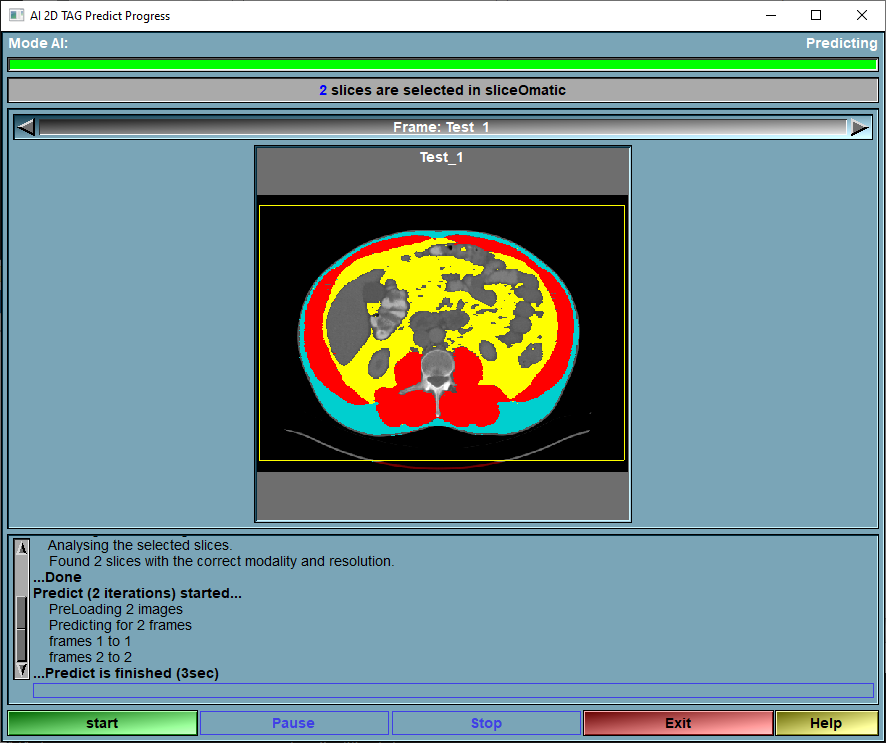
Progress Bar |
Show the progression of the predicting
|
Slice status |
This line will tell you how many slices are currently selected in sliceO and are available for the prediction.
|
Slice selection |
You can select any of the available slices for preview and ROI placement.
|
Image preview |
The slice selected with the "Slice selection" tool is displayed here. If the ROI of the training is smaller than the FoV of the slice, you will see a yellow box representing the ROI of the training on the image. You can place this ROI by simply clicking in the box and sliding it to the desired position.
|
|
Text Feedback |
Report some info on the progression of the predictions.
|
|
Start |
Start the computation of the prediction.
|
|
Pause/Resume |
Pause/resume the computation.
|
|
Stop |
Stop the computation.
|
|
Exit |
Exit this page.
|
Help |
Display this web page. |
The Python files
You can add your own metrics and models to this mode. You just have to follow the syntax described here:
The Python directory.
All the Python files used by sliceOmatic's AI module are stored in the Python directory. By default this is in "c:\Program Files\TomoVision\SliceO_Python". The location of this directory can be changed through the sliceOmatic's "Config" interface.
The Metrics Python files.
For my metrics files, I use names that start with "metrics ", but the name is not really important. What is important is that the file contain either a "metrics_2D" function, a "loss_2D" function or both.
You can have 3 types of metrics functions
The "Loss" metrics:
- The Loss functions compute a loss metrics used to train the AI.
The value of the loss function must decrease when we are approach perfect results.
The name of the loss function must be: "loss_2D_TAG" and have 2 arguments: "y_true" and "y_pred", 2 tensors, as described in Keras doc.
You must define a flag for the function: loss_2D_TAG.flag =... (The choices are between: "mean" "weighted" and "class" )
You must define the name of the function: loss_2D_TAG.__name__ =...
You must define a version for the function: loss_2D_TAG.__version__ =... (The version syntax is: "major.minor". ex: "2.3")
You must define the description of the function: loss_2D_TAG.description =...
|
|
import keras as kr
# ---------------------------------------------------- # The function must be called "loss_2D_TAG" # ---------------------------------------------------- def loss_2D_TAG( y_true, y_pred ) :
# --- We simply call the Keras function --- return( kr.losses.categorical_crossentropy( y_true, y_pred ) )
# ---------------------------------------------------- # Give a name for this metrics # ---------------------------------------------------- loss_2D_TAG.__name__ = "Categorical CrossEntropy"
# ---------------------------------------------------- # Give a version for this metrics # ---------------------------------------------------- loss_2D_TAG.__version__ = "2.1" # ---------------------------------------------------- # Give a name for this metrics # ---------------------------------------------------- loss_2D_TAG.description = "Call the Keras \"categorical_crossentropy\" function:\n" \ "Computes the crossentropy loss between the labels and predictions." |
You can have 2 types of metrics: "global" or "Per class".
The "global" metrics:
- The Metrics functions compute a metrics used as feedback when training or testing.
The name of the metrics function must be: "metrics_2D_TAG" and have 2 arguments: "y_true" and "y_pred", 2 tensors, (as described in Keras doc.)
You must define a flag for the function: metrics_2D_TAG.flag =... (The choices are between: "mean" "weighted" and "class" )
You must define the name of the function: metrics_2D_TAG.__name__ =...
You must define a version for the function: metrics_2D_TAG.__version__ =... (The version syntax is: "major.minor". ex: "2.3")
You must define the description of the function: metrics_2D_TAG.description =...
|
|
|
The "per class" metric:
The name of the metrics function must be: "metrics_2D_TAG" and have 2 arguments: "class_idx" and "name", the index and name of the target class, for "Per class" metrics.
The "per class" metrics return a "global" metric function for the desired class.
You must define the name of the function: metrics_2D_TAG.__name__ =...
You must define a version for the function: metrics_2D_TAG.__version__ =... (The version syntax is: "major.minor". ex: "2.3")
You must define the description of the function: metrics_2D_TAG.description =...
You must also define a "flag" that must contain the string "class". (metrics_2D_TAG.flag = "class")
|
|
|
The Model Python files.
Again, I use the prefix "model " for my models files but the name is no important. The important is that the file contain a "model_2D_TAG" function.
That function receive 4 arguments: dim_x, dim_y, dim_z and num_classes. dim_x and y are the X and Y resolution of the images we will train this model with and num_classes is the number of classes. The "dim_z" argument is not used in 2D models. The function must define the layers of your model and return the "model" variable returned by the Keras "Model" function.
You must define the name of the function: model_2D_TAG.__name__ =...
You must define a version for the function: model_2D_TAG.__version__ =... (The version syntax is: "major.minor". ex: "2.3")
You must define the description of the function: model_2D_TAG.description =...
|
|
|
The Test Python files.
By default, I test for the presence of Python, Numpy, Tensorflow and Keras. If you use another module in your Python code, you can add a new test file. SliceO will use this to test that the desired module is indeed loaded when it start the AI module.
The file must contain a "version" function that return the version number for the target module.
It must also contain a "__name__" and a "__version__" definition.
|
|
|
Accessing sliceOmatic variables from Python.
You can access any of the sliceOmatic variables from your python code.
The functions for this are:
sliceO_Var_Get_Int( Variable_Name )
sliceO_Var_Get_Float( Variable_Name )
sliceO_Var_Get_Str( Variable_Name )
return one (or an array of) value(s), depending on the variable.
sliceO_Var_Set_Int( Variable_Name, Value )
sliceO_Var_Set_Float( Variable_Name, Value )
sliceO_Var_Set_Str( Variable_Name, Value )
Assign the value "Value" to the variable "Var_Name". At this time only variable with one value can be "Set" (no arrays).
From the Display Area
There is no display area interaction specific to this mode.
From the Keyboard
The following commands are mapped to keyboard keys as a shortcut:
|
|
|
|
|
|
Key map |
Action |
|
|
|
|
|
|
F1 |
Set the color scheme mode for all windows: F1=Grey, F2=Mixed, F3=Tint and F4=Over |
|
|
F2 |
|
|
|
F3 |
|
|
|
F4 |
|
|
|
|
|
|
|
|
From the Command Line
System Variables defined in this library:
|
|
$AI_RES_X |
(I16) |
|
|
|
$AI_RES_Y |
(I16) |
|
|
|
$AI_RES_Z |
(I16) |
|
|
|
$AI_RES_MULT |
(I16) |
All resolutions will be a multiple of this value (def=16). This constraint is imposed by U-NET |
|
|
$AI_CLASS_NB |
(I16) |
|
|
|
$AI_CLASS_LABEL |
A(W) |
* $AI_CLASS_NB |
|
|
$AI_CLASS_RATIO |
A(F32) |
* $AI_CLASS_NB |
|
|
$AI_CLASS_WEIGHTS |
A(F32) |
* $AI_CLASS_NB |
Tversky metrics parameters:
|
|
$AI_TVERSKY_ALPHA |
(F32) |
|
|
|
$AI_TVERSKY_BETA |
(F32) |
|
TAG re-mapping:
|
|
$AI_TAG_MAP_IN_NB |
(I32) |
|
|
|
$AI_TAG_MAP_IN_VAL |
A(U8) |
* $AI_CLASS_NB |
|
|
$AI_TAG_MAP_OUT |
A(U8) |
* $AI_CLASS_NB |
Training Parameters:
|
|
$AI_TRAIN_STEP_MAX |
(I32) |
|
|
|
$AI_TRAIN_STEP_CUR |
(I32) |
|
|
|
$AI_TRAIN_EPOCH_MAX |
(I32) |
|
|
|
$AI_TRAIN_EPOCH_CUR |
(I32) |
|
|
|
$AI_TRAIN_BATCH_MAX |
(I32) |
|
|
|
$AI_TRAIN_BATCH_CUR |
(I32) |
|
|
|
$AI_TRAIN_LR |
(F32) |
|
|
|
$AI_TRAIN_EARLY_FLAG |
(I32) |
|
|
|
$AI_TRAIN_EARLY_NB |
(I32) |
|
Python Variables:
|
|
$PYTHON_FLAG |
(U32) |
|
|
|
$PYTHON_MODULE_PATH |
(W) |
|
|
|
$PYTHON_INTERPRETER_PATH |
(W) |
|
|
|
$PYTHON_SLICEO |
(P) |
|
|
|
$PYTHON_TEMP |
(W) |
|
Commands recognized in this mode:
Python: path "path"
Python: temp "path"
A2T: file read "path"
A2T: file "path" (on|off)
A2T: preproc resolution x [y]
A2T: preproc modality value
A2T: preproc min value
A2T: preproc max value
A2T: preproc norm ("HU" | "min-max" | "z-score")
A2T: class nb value
A2T: class in id value
A2T: class out id value
A2T: class label id "label"
A2T: augment "name" (on|off) value
A2T: metrics loss "name"
A2T: metrics feedback clear
A2T: metrics feedback "name"
A2T: split test value
A2T: split mode value
A2T: split split value
A2T: split kfold value
A2T: model cur "name"
A2T: model modality value
A2T: model class value
A2T: weights cur "name"
A2T: weights load