In this step, you will read the files needed to select and find the target slice at L# into the sliceOmatic program.
If you already know the exact file containing the L3 slice, you can simply drag&drop that file on sliceOmatic and bypass step 2.
The Interface:
In this step, sliceOmatic is placed in Mode "DB File management".
Only one image window is displayed and it is in "Mode All".
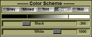
The "Color Scheme" tool is open.
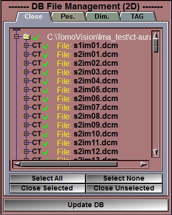
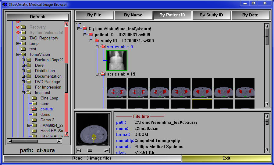
The "DICOM Browser" is open.
What to do:
|
|
First, if you have any previously loaded files, you can close them using the "DB File Management" interface.
•First, click on the "Select All" button
•Then, click on the "Close Selected" button
•Finally, click on the "Update DB" button |
|
|
|
You can use the DICOM Browser to select the study you will analyze. |
|
|
|
You can find step by step instructions by following this link.
In this version of the protocol, you only need to load axial slices. You no longer need any pilot, scout images, sagittal or coronal slices. So you should limit the slices you load to a single series, or even just some slices around L3. |
|
Or, you can simply drag & drop the desired files directly on the sliceOmatic's window.
Note:
|
|
You should limit the files you read to the axial slices around L3. Make sure to take in enough slices to be able to identify the L3 slices from the sagittal view, but no need to take in more than 3 to 4 vertebra. |
|
All the read files will be visible in the sliceOmatic's window.
|
|
You can decrease/increase the size of the displayed images with the "+" and "-" keys on the keyboard.
|
|